Why Contrastive Learning Is Basically the Backbone of Visual Language Models

Visual Language Models (VLMs) kind of feel like magic when you first use them. You upload a photo of a specific car part or a rare tropical fruit, ask “What is this?” in normal English, and it just answers. No hesitation. No error message about unsupported categories.

But honestly, behind that apparent intelligence is a pretty simple idea. It’s not about memorizing what things look like pixel-by-pixel. It’s about learning by comparing. About understanding relationships rather than rigid definitions.

That idea is called Contrastive Learning, and it is the real engine running modern AI. If you want to understand how we got from “dumb” image classifiers stuck recognizing 1,000 objects to smart models like GPT-4o that can discuss abstract art, you have to understand this shift.

Table of Contents

1. The Old Way: Vision Trained on Fixed Lists

2. The Big Shift: Learning Relationships Instead of Labels

3. How It Actually Works: The Magnet Analogy

4. The Mathematical Intuition (Without the Scary Math)

5. Why This Matters: Breaking Out of the “Closed World”

6. Zero-Shot Learning: The Killer Feature

7. Why It Scales: The Internet is the Dataset

8. The Compositional Understanding Problem

9. Real-World Impact: What Changed Because of This

10. It’s Not Perfect Though

11. The Bottom Line

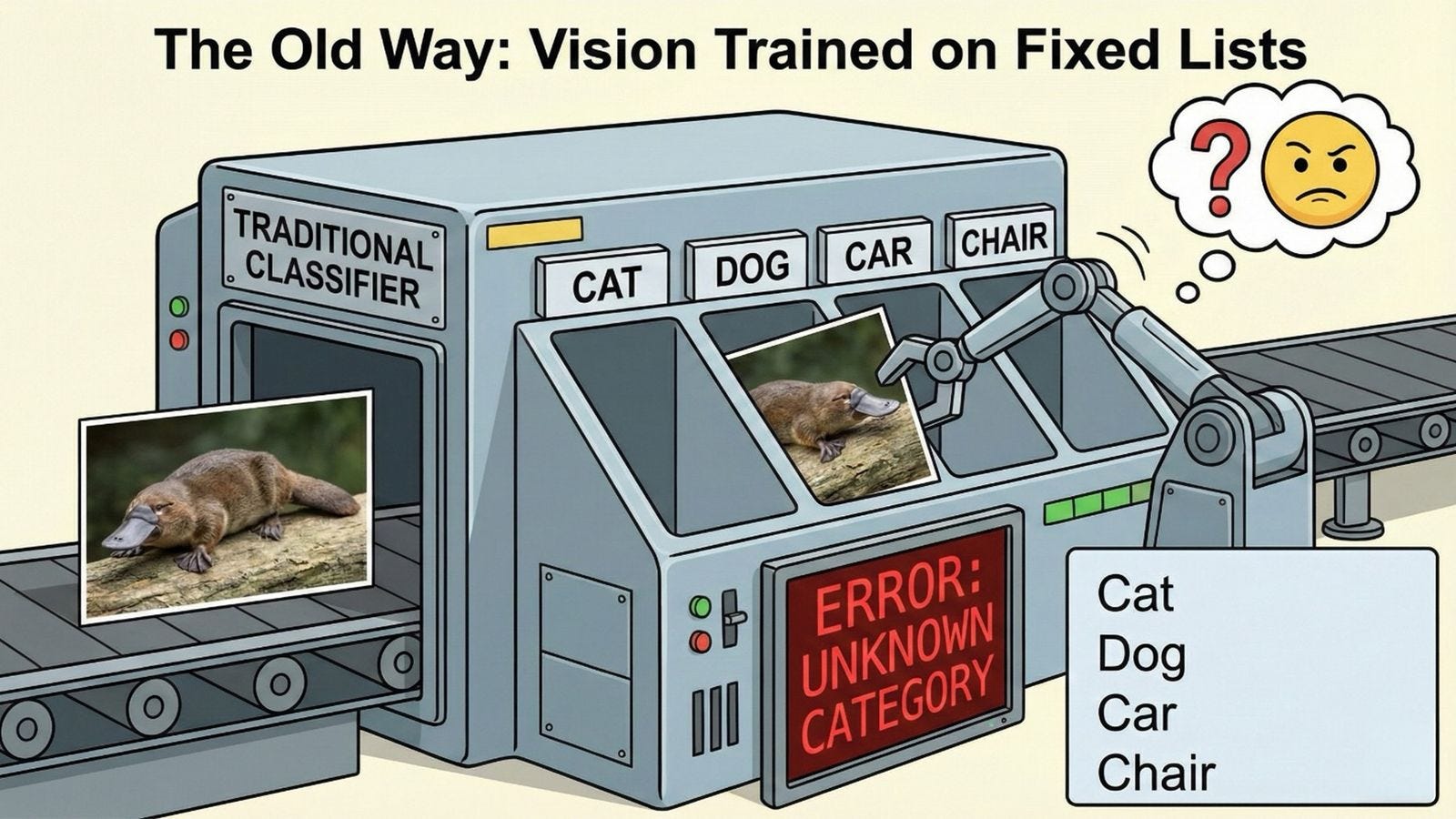
1. The Old Way: Vision Trained on Fixed Lists

Back in the day (like, 2018, which is ancient history in AI years), traditional computer vision models learned in a super constrained way. It was basically a multiple-choice test for computers, except the computer could never skip a question or write “I don’t know.”

You fed an image in. A label came out.

• Cat

• Dog

• Car

• Chair

The model’s whole understanding of the world was limited to those predefined categories, usually from a dataset like ImageNet with around 1,000 labels. Think of it like a mail sorter with exactly 1,000 slots, numbered and labeled at the factory. If you mailed a “platypus” but the sorter only had slots for “beaver” and “duck,” the machine would panic. It would pick whichever looked closest, even if neither was remotely correct. It literally couldn’t see the platypus as a platypus because it didn’t have a slot for it.

This worked okay for specific, narrow tasks, like spotting stop signs in autonomous driving or flagging explicit content. You could get 95%+ accuracy if your problem fit neatly into those predefined boxes.

But it didn’t scale to the real world. The real world is messy, infinite, and constantly evolving. You can’t make a list of every single object, scene, concept, style, or variation that exists. What about “a rusty stop sign covered in graffiti”? What about “abstract expressionist painting in the style of Rothko”? What about “a meme showing a confused cat looking at a salad”?

The old paradigm broke down because the world doesn’t come with fixed labels. And humans certainly don’t experience vision that way. When you see something new, you don’t fail because it’s not in your mental catalog. You describe it, compare it to things you know, and figure it out through context.

2. The Big Shift: Learning Relationships Instead of Labels

Contrastive learning flips the problem upside down in a way that feels obvious in retrospect but was revolutionary at the time.

Instead of asking “What label does this image belong to?”, the model asks: “Which text description matches this image best?”

And just as important, it asks: “Which texts do not match this image?”

It turns learning into a game of “Spot the Difference” or “Match the Pair” rather than strict memorization. The model looks at an image and a bunch of text snippets and tries to figure out which ones naturally go together and which ones don’t.

This is huge because it mirrors how humans actually learn language and visual concepts as children. You don’t memorize a lookup table. You hear “That’s a dog” while looking at a dog dozens of times across different contexts (big dogs, small dogs, dogs running, dogs sleeping) and your brain learns the pattern, the essence of “dog-ness,” by contrast with “not-dog” things.

The insight here is profound: meaning emerges from relationships, not from definitions. A dog is a dog not because of some intrinsic “dog ID tag” but because it’s more similar to other dogs than it is to cats, horses, or bicycles. Language works the same way. The word “dog” gets its meaning from how it’s used differently from “cat,” “puppy,” “wolf,” etc.

Contrastive learning operationalizes this insight at scale.

3. How It Actually Works: The Magnet Analogy

You don’t need to know the complex math to get the intuition, though we’ll peek under the hood in the next section. For now, think of it like magnets.

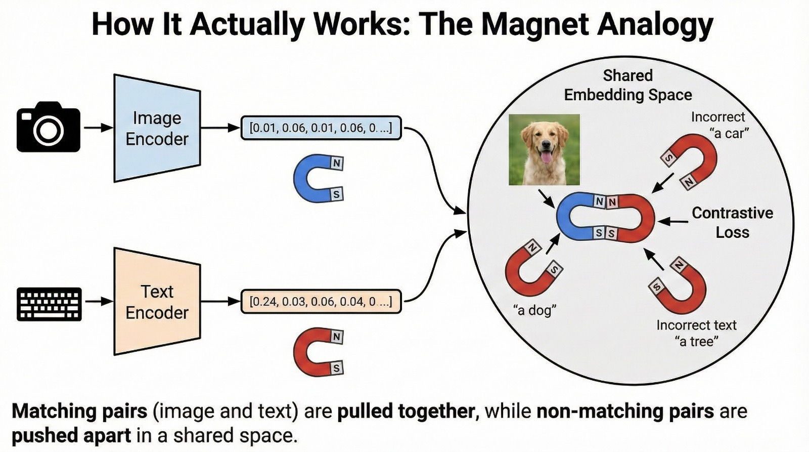
At a high level, models like CLIP (Contrastive Language-Image Pre-training) use two encoders:

Image Encoder: Turns a picture into a list of numbers (a vector). Think of it as a 512-dimensional or 1024-dimensional “fingerprint” of the image.

Text Encoder: Turns text into a list of numbers in that same dimensional space.

Why Two Separate Encoders?

The encoders start with different architectures because images and text are fundamentally different data types. Vision typically uses convolutional networks or transformers adapted for 2D structure, processing pixels arranged in grids. Text uses transformer models built for sequential tokens, processing words in order.

But here’s the key: they project into the same shared space, which is what enables comparison. The training process forces these very different data types to speak the same mathematical language. It’s like having a Spanish speaker and a Mandarin speaker both learning to communicate through a universal intermediate language.

What Do “Dimensions” Actually Mean?

When we say “512-dimensional vector,” what does that mean? Each dimension captures some learned aspect of the image or text. Some dimensions might loosely correspond to concepts we recognize - maybe something like “furriness,” “metallic-ness,” or “outdoor-ness” - but most represent abstract patterns we can’t easily name. The model discovers these dimensions on its own through training. Think of them as 512 different ways to measure and describe what’s in an image or text.

The Projection Head: The Final Translation Layer

After the encoders create their initial representations, the vectors pass through an additional small neural network called a “projection head.” This final layer maps the representations into the actual shared embedding space where comparison happens. Think of it as a translator ensuring both modalities end up speaking exactly the same dialect, with the same vocabulary and grammar rules.

The image encoder might naturally produce vectors that emphasize visual texture and color, while the text encoder emphasizes semantic relationships between words. The projection heads reshape these into a common format where direct comparison makes sense.

The Magic Happens in Training

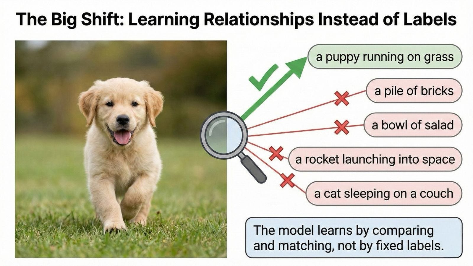
The model takes an image (say, a photo of a golden retriever puppy running on grass) and pairs it with the correct caption: “a puppy running on grass.” This is a positive pair.

The training objective is simple but powerful: pull these vectors closer together. Like the north and south poles of a magnet snapping together, the model adjusts its internal parameters so that the numerical representation of the image and the numerical representation of the text become more similar.

At the same time, it looks at that puppy photo and compares it to random captions from other images in the batch: “a pile of bricks,” “a bowl of salad,” “a rocket launching into space.” These are negative pairs.

The model pushes their vectors far apart, like two north poles repelling each other. You want maximum distance between things that don’t match.

How Batching Creates Scale

Here’s where the efficiency becomes remarkable. In a training batch of, say, 32,768 images with their corresponding captions, you automatically get 32,768 positive pairs (each image with its correct caption). But you also get 32,768 × (32,767) = over 1 billion negative pairs - every image compared against every other caption in the batch.

This massive number of comparisons happens in parallel, which is why modern contrastive learning requires serious computational power but scales so efficiently. The model isn’t doing billions of separate training steps. It’s doing one batch where billions of comparisons influence the learning simultaneously.

The Iterative Refinement Process

This isn’t a one-shot comparison. The model adjusts millions of internal weights slightly after each batch, following the gradient that reduces the loss - the mathematical measure of how wrong the current predictions are. Over thousands of batches and billions of examples, something remarkable emerges: a shared embedding space. A mathematical landscape in which images and language coexist.

In this space, a photo of a golden retriever ends up right next to the phrase “a dog playing outside.” That cluster sits near “puppy,” “retriever,” “pet.” It’s far away from “sports car,” “skyscraper,” or “quantum physics.”

The model isn’t memorizing. It’s building a map of meaning through pure comparison.

4. The Mathematical Intuition (Without the Scary Math)

If you’re curious about what’s happening under the hood, here’s the simplified version.

The core function is called a contrastive loss, often specifically the InfoNCE loss. Don’t worry about the name. Here’s what it does:

For each image in a batch, the model calculates how similar it is to every text description using a similarity metric (usually cosine similarity, which is basically the angle between two vectors).

Why Cosine Similarity Specifically?

Cosine similarity measures the angle between vectors, ignoring their magnitude. This matters because we care about direction in the embedding space (is this vector pointing toward “dog-ness”?) not absolute size (how “loud” is the signal?).

Imagine two vectors as arrows pointing in different directions. If they point the same way, they’re similar (cosine similarity = 1). If they point opposite ways, they’re dissimilar (cosine similarity = -1). If they’re perpendicular, they’re unrelated (cosine similarity = 0).

This normalization is crucial. It means the model won’t be confused by irrelevant factors like image brightness (which might make all the pixel values bigger) or text length (which might make the text vector longer). We only care about the semantic direction.

The Push-Pull Dynamic

The model wants high similarity for the correct image-text pair and low similarity for all the incorrect pairs. The loss function penalizes the model whenever a correct pair isn’t similar enough or an incorrect pair is too similar.

This creates a push-pull dynamic. During training, the model is constantly adjusting to maximize the gap between matches and non-matches. It’s learning discriminative features. What makes a dog distinctly a dog, not just in general, but specifically when contrasted with not-dog things.

Bidirectional Symmetry

The contrastive loss is symmetric - it pulls both the image toward the text AND the text toward the image. This bidirectionality is crucial. It means you can later search in either direction: find images matching text OR find text matching images. This symmetry is what enables reverse image search, visual question answering, and text-to-image retrieval. The relationship works both ways.

The Temperature Parameter: Controlling Confidence

There’s one more dial that significantly affects learning: the temperature parameter (often written as τ in papers).

The model uses this “temperature” setting to control how confident it needs to be. A low temperature means the model is forced to make sharp distinctions - the correct pair must be WAY more similar than wrong pairs. The model becomes very decisive, almost black-and-white in its judgments.

A high temperature is more forgiving, allowing softer boundaries. The model can be more uncertain, accepting that some incorrect pairs might be somewhat similar to the correct one. This is useful early in training when the model is still figuring things out.

This seemingly minor dial has huge effects on what the model learns. Too low, and the model might overfit to small details. Too high, and it might learn too coarse representations that miss important distinctions.

The Power of Ranking

What makes this different from traditional supervised learning is that you’re not teaching the model a single “correct answer.” You’re teaching it to rank options. Given this image, is it more like “a beach at sunset” or “a crowded subway car”? The model learns through millions of these comparative judgments.

This ranking approach is surprisingly robust. Even if the caption isn’t perfect (maybe it says “a dog” when it’s technically a wolf), the model still learns something useful because “a dog” is far more correct than “a helicopter.”

Hard Negatives: The Challenging Comparisons

Not all negative pairs are equally useful for learning. “A puppy” vs. “a rocket ship” is an easy distinction - too easy to be informative. The model learns more from hard negatives: “a puppy” vs. “a kitten” or “a wolf cub.”

These challenging comparisons force the model to learn fine-grained differences. What specifically makes a puppy different from a kitten, beyond just being a young furry animal? Advanced implementations actively mine for these hard negatives during training, deliberately finding the most confusable examples to show the model.

Think of it like studying for a test. You don’t learn much from questions that are obviously wrong. You learn from the tricky ones that require careful thought.

5. Why This Matters: Breaking Out of the “Closed World”

Here’s the philosophical importance that’s easy to miss: traditional vision models lived in a closed world. They operated on the assumption that every possible input could be assigned to one of the predefined categories. This is called the “closed-world assumption” in AI.

But the real world is an open world. New things appear constantly. New slang, new fashion trends, new memes, new products, new art styles. A model trained in 2020 on fixed labels would be completely blind to anything that emerged afterward.

Contrastive learning is what unlocks open-vocabulary recognition.

You could build the biggest vision model in history with billions of parameters, but without this contrastive alignment to language, it would still be trapped. It could only see the things it was explicitly taught.

With contrastive learning, the model can recognize things it’s never seen explicitly labeled because it learned the deeper compositional structure of both vision and language.

It knows what “fluffy” looks like. It knows what “cat” looks like. So even if it never saw the exact phrase “fluffy cat” during training, it can infer what that should look like by combining concepts.

This is the difference between memorization and understanding. Or at least, it’s one step closer.

6. Zero-Shot Learning: The Killer Feature

This is where contrastive learning goes from “interesting technique” to “this changes everything.”

Zero-shot learning means the model can perform a task it was never explicitly trained to do. No fine-tuning. No labeled dataset. Just pure inference from its learned representations.

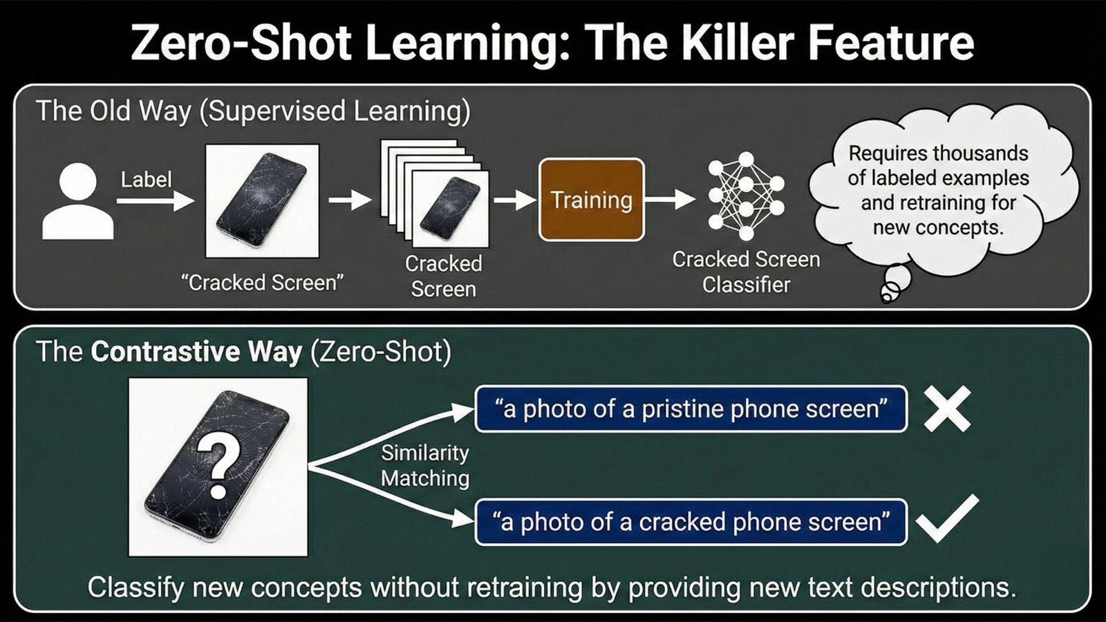
Let’s say you want to build a detector for “cracked iPhone screens” for quality control in a repair shop.

The Old Way:

You’d have to gather 5,000+ photos of cracked screens. Hire people to label them by hand. Train a custom model (expensive, time-consuming). Hope your model generalizes to crack patterns it hasn’t seen. Realize you need more data when it fails on edge cases. Repeat.

The Contrastive Way:

Feed the VLM an image. Give it two text prompts: “a photo of a pristine phone screen” and “a photo of a cracked phone screen.” The model checks its internal embedding space. Is this image vector closer to the “pristine” text vector or the “cracked” text vector? Done.

Boom. You have a functional classifier. No new labels. No training time. No GPUs running for days. Just comparison.

This works for anything you can describe in language:

• “A photo of a counterfeit product” vs. “an authentic product”

• “A medical scan showing a tumor” vs. “a healthy scan” (though you’d want validation)

• “A Renaissance painting” vs. “an Impressionist painting”

• “A parking lot that’s mostly full” vs. “a parking lot that’s mostly empty”

The implications are staggering. You can spin up new applications in minutes that would have taken months with old-school supervised learning. This is why VLMs have exploded in adoption across industries.

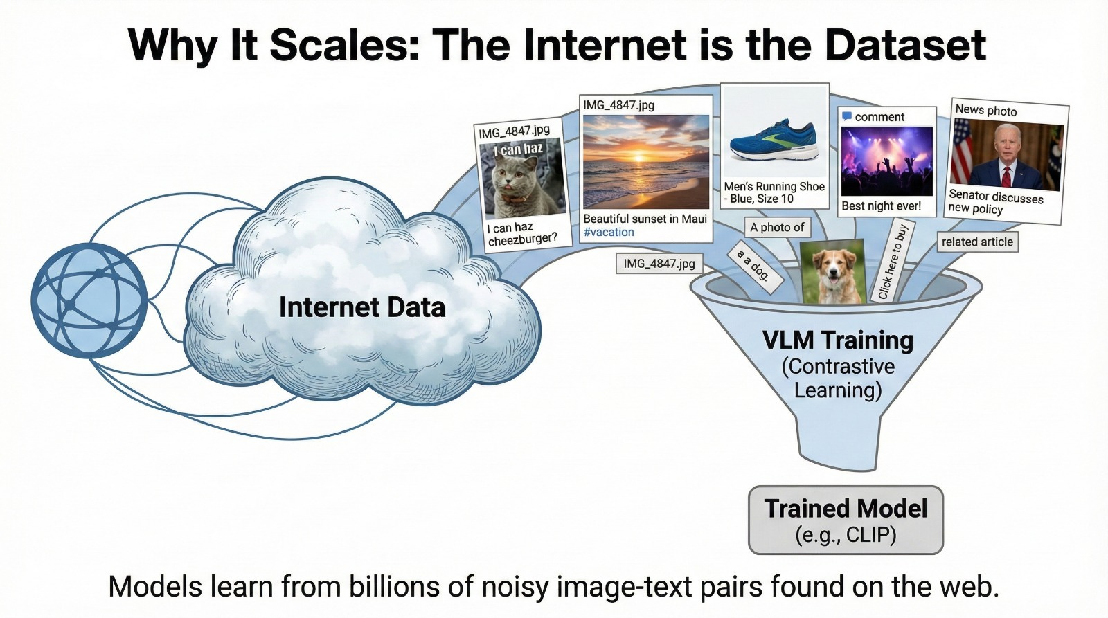
7. Why It Scales: The Internet is the Dataset

There’s a practical reason this technique dominates the modern AI landscape: data abundance.

Old models needed humans to painstakingly annotate data. Drawing bounding boxes around objects. Labeling images one by one. Categorizing, tagging, quality-checking. This is expensive (crowd workers or expert annotators), slow (human bottleneck), error-prone (labeling is subjective and tiring), and non-scalable (you can’t label the entire internet).

But contrastive learning runs on the internet itself. There are billions of images online with captions, alt text, titles, or surrounding context. They aren’t perfect. Many are noisy, vague, or just plain wrong. “IMG_4847.jpg” isn’t a great caption. But they’re abundant.

The Key Insight: Noise Tolerance

The model tolerates noise really well because the learning is relative.

The caption doesn’t need to be perfect poetry. It doesn’t even need to be 100% accurate. It just needs to match the image better than a random sentence does.

When you’re training on millions of examples simultaneously, the noise averages out - assuming the noise is random and unbiased. The correct patterns strengthen through repetition while the random errors cancel out statistically.

However, there’s an important caveat: systematic biases don’t average out. If most images of doctors show men and most images of nurses show women (which they do on the internet), that bias accumulates rather than cancels. The model learns the bias as if it were truth. We’ll come back to this in the limitations section.

Data Augmentation: Teaching Invariance

The model also sees the same image with different augmentations - crops, color shifts, rotations, blurring, contrast changes. This teaches it to focus on semantic content rather than superficial details. A dog is still a dog whether the photo is bright or dim, centered or cropped, shot from above or from the side.

This augmentation strategy is crucial for generalization. Without it, the model might learn that “beach” always means bright sunny photos, failing to recognize a beach on a cloudy day.

The Internet as a training ground

This allows companies to train on massive, messy datasets scraped from the web. Datasets that would completely break a traditional supervised model. CLIP was trained on 400 million image-text pairs from the internet. You could never hand-label that many images. But you can leverage existing structure on the web.

The internet becomes your training set. Humanity’s collective captioning effort (every Instagram post, every Wikipedia image, every product description) becomes machine learning fuel.

8. The Compositional Understanding Problem

Let’s go deeper on something subtle but crucial: compositional generalization.

Human language is compositional. We can understand “blue car” even if we’ve never seen those exact two words together, because we know “blue” and “car” separately. We can parse “a dog wearing sunglasses riding a skateboard” even though we’ve probably never seen that exact scene before.

Contrastive learning gives models a primitive version of this superpower.

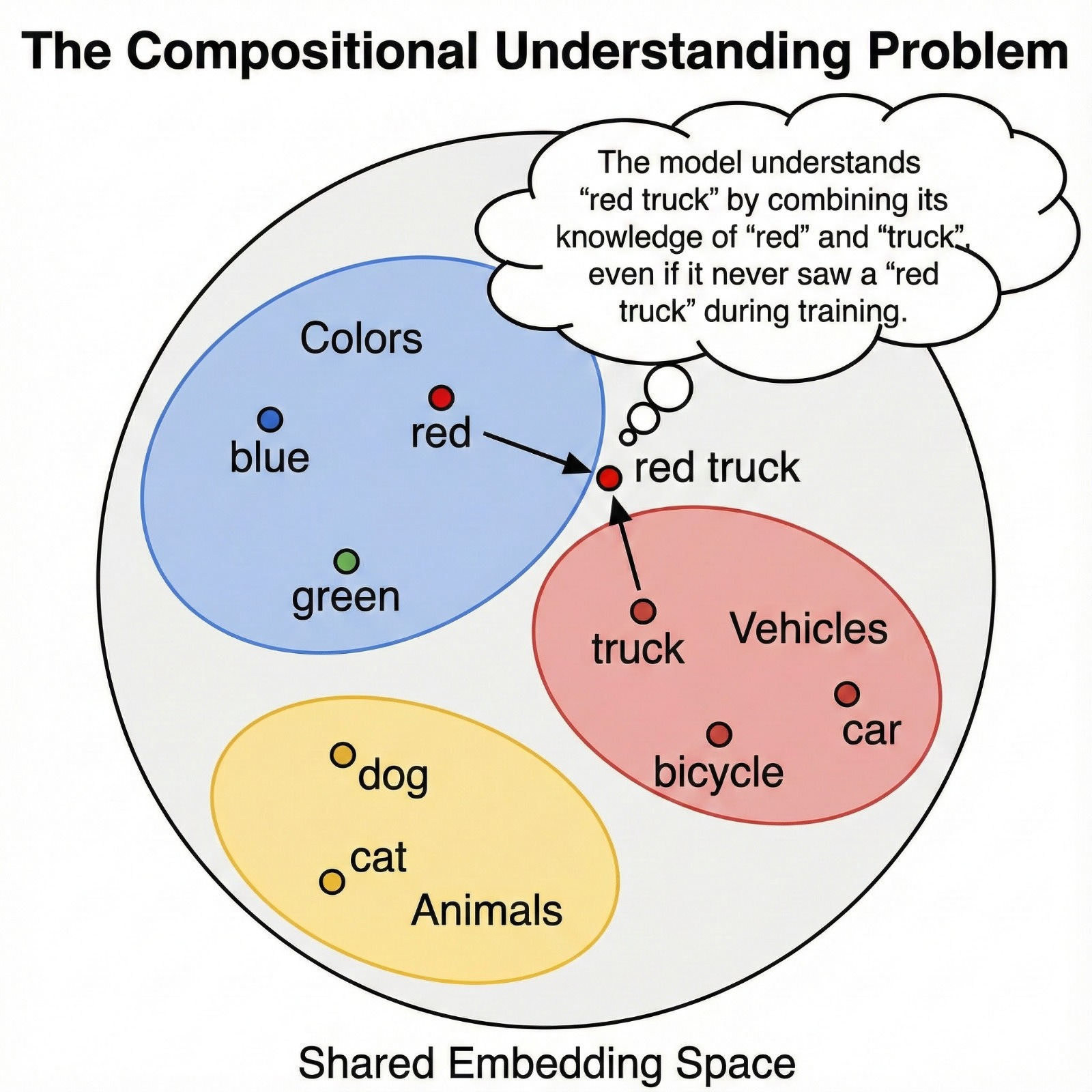
Because the model learned visual features and text features in a shared space, it can combine concepts in novel ways. If it learned what “red” looks like (from “red apple,” “red car,” “red sunset”) and what “truck” looks like (from “delivery truck,” “pickup truck,” “fire truck”), then it can infer what “red truck” should look like, even if it never saw that exact phrase during training.

The Geometry of Meaning

The embedding space has surprising geometric properties. Concepts cluster together. There’s a “region” for animals, a “region” for vehicles, a “region” for emotions. Similar concepts end up near each other not because anyone programmed it that way, but because they appeared in similar contexts during training.

Sometimes vector arithmetic even works: the vector for “dog” minus “puppy” plus “cat” can land near “kitten.” The relationship “puppy is to dog as kitten is to cat” emerges naturally in the geometry. This isn’t guaranteed - the space isn’t perfectly linear—but these regularities emerge from pure comparison, which is remarkable.

Imagine a 2D projection of the embedding space: dog photos cluster in one region, cat photos nearby, vehicle photos in a different area entirely, and landscape photos in yet another zone. Text descriptions live in these same regions. “A happy dog” sits right in the dog cluster. “A red sports car” sits in the vehicle zone. The spatial organization encodes semantic similarity.

Not Just Memorization

This is different from memorization. The model isn’t retrieving “red truck” from a database. It’s computing it by navigating the embedding space, finding where “red-ness” and “truck-ness” intersect.

This compositional ability isn’t perfect (more on limitations later), but it’s the reason these models feel “smart” rather than just being giant lookup tables. They can handle combinatorial explosion. With just 1,000 visual concepts and 1,000 descriptive words, you can theoretically compose millions of meaningful combinations.

9. Real-World Impact: What Changed Because of This

Let’s talk impact, because this isn’t just academic. Contrastive learning fundamentally changed what’s possible in production AI systems.

Content Moderation: Companies like Meta and Google use VLMs to detect policy-violating content without manually defining every single violation. Instead of training separate models for “hate symbols,” “graphic violence,” “self-harm,” etc., they can describe the concept in text and let the model match.

Accessibility: Alt-text generation for blind users improved dramatically. Instead of generic labels like “outdoor scene,” VLMs can generate descriptive captions like “a person in a red jacket standing on a mountain overlook at sunset.”

E-commerce Search: You can now search product catalogs with natural language (”comfortable running shoes under $100”) or even upload a photo (”find me this but in blue”). Traditional search required exact keyword matches or manual tagging.

Medical Imaging: Radiologists can query image databases with descriptions of what they’re looking for, and the model can surface relevant cases even without explicit diagnostic labels.

Creative Tools: Design software like Photoshop uses VLMs to enable text-based selection (”select all the plants in this image”) without manual masking.

Manufacturing Quality Control: Factories use VLMs to detect defects by simply describing what a defect looks like, rather than collecting thousands of labeled examples of each possible failure mode.

Wildlife Conservation: Researchers can search camera trap footage for specific animal behaviors or rare species using text descriptions, dramatically speeding up ecological studies.

All of these applications share a common thread: flexibility. The model adapts to your needs through language, rather than requiring months of custom training for each use case.

The Broader Multimodal Vision

The same principle extends beyond just vision and language. Modern models use contrastive learning to align audio, video, 3D shapes, sensor data, protein structures—any modality that can be encoded numerically.

Imagine asking “find me video clips where someone sounds frustrated” and the model can search audio. Or “show me 3D models similar to this chair design” and it understands shape. The dream is a universal embedding space where any type of data can be compared to any other type, all searchable and combinable through natural language.

We’re not fully there yet, but contrastive learning paved the road.

10. It’s Not Perfect Though

Let’s be honest about the limitations, because understanding what contrastive learning can’t do is just as important as understanding what it can.

Fine-Grained Details Suffer

Since the model learns from web-scale captions, it focuses on the overall “vibe” or main subject. People don’t caption images with precise details. You get “a bird on a branch,” not “a juvenile male house sparrow perched on an oak tree branch.”

This means:

Counting is surprisingly hard. “How many apples are in this bowl?” often gets wrong answers. The model learned “apples” as a concept but didn’t learn numeracy through image-text pairing. Captions rarely specify exact quantities.

Spatial relationships are tricky too. “Is the cup to the left or right of the spoon?” can confuse models. Captions rarely specify precise spatial layouts. They say “a cup and spoon on a table” but not “a cup to the left of a spoon.”

Subtle distinctions fail. Telling apart similar species of birds or breeds of dogs requires fine-grained visual features that get washed out in the coarse-grained contrastive objective. The model knows “bird” really well, but “house sparrow vs. song sparrow” is much harder.

Some newer architectures that incorporate attention mechanisms over spatial regions are improving here, but it remains a challenge.

Association ≠ Understanding

The model knows “astronaut” and “horse” go together visually because it saw sci-fi art or memes during training. But it doesn’t truly understand the physics of why a horse can’t actually survive in space. It’s pattern matching, not reasoning.

Similarly, it might associate “beach” with “sunny” because most beach photos online show sunny weather, failing to recognize a foggy beach as still being a beach.

Bias Amplification

Because training data comes from the internet, all of the internet’s biases come along for the ride. Stereotypical associations (doctors are men, nurses are women, CEOs are older white men, etc.) get baked into the embedding space.

This is particularly insidious because the biases aren’t explicitly programmed - they emerge from the statistical patterns in the training data. The model learns what the internet shows it, and the internet reflects historical and ongoing societal biases.

Addressing this requires careful dataset curation, debiasing techniques, and acknowledgment that “learning from the internet” means inheriting its flaws along with its knowledge.

Literal Text in Images

Ironically, models trained this way can struggle with actual text that appears within images. A photo of a “STOP” sign might not register the text “STOP” as strongly as the octagonal red shape, because the model learned visual-linguistic alignment between images and captions, not OCR (optical character recognition).

The image encoder treats letters as visual patterns, not linguistic symbols. To truly “read” text in images, you need additional training specifically on that task.

The Loss Function’s Blind Spots

Contrastive learning optimizes for similarity matching. If two very different images both match the same vague caption equally well, the model might not learn to distinguish them. This can lead to mode collapse (where the model learns overly generic representations) or feature neglect (where certain visual attributes are ignored).

For example, if most captions say “a person” without mentioning age, ethnicity, or clothing, the model might not learn to encode those attributes as strongly, even though they’re visually present.

11. The Bottom Line

Here’s what you need to remember, whether you’re a beginner, a practitioner, or just someone trying to understand where AI is heading:

Visual Language Models aren’t impressive because they “see better” than old models. In fact, sometimes their raw pixel-level vision is technically worse than specialized classifiers trained for specific tasks.

They’re impressive because they compare better. They connect the dots between what things look like and what words mean.

This distinction matters. It means the future of AI isn’t about building bigger isolated models. It’s about building models that connect modalities through shared representations.

Language becomes the universal interface. It’s not just an add-on. It’s the core enabler that makes vision models useful, flexible, and general.

We’re moving from brittle, task-specific AI to fluid, task-agnostic AI that you can steer with words. You don’t need to retrain a model to recognize a new object class. You just describe it. The model finds it in the embedding space it already learned.

The Core Insight

If you understand contrastive learning, you understand why CLIP changed computer vision forever. You understand why multimodal models like GPT-4o can discuss images fluently. You understand why companies are racing to build bigger VLMs rather than better single-task classifiers.

Contrastive learning isn’t just a training trick. It’s the backbone of modern AI’s ability to bridge perception and language.

And once you see it, you can’t unsee it. Every time you upload an image to a chatbot and it “gets it,” you’re watching contrastive learning in action. Millions of learned comparisons crystallizing into what feels like understanding.

That’s the real magic. Not that the model knows everything, but that it learned how to compare anything to anything else. And in that comparison, meaning emerges.

The model doesn’t just recognize objects. It understands - in its limited, statistical way - the relationships between visual concepts and linguistic descriptions. It built a bridge between seeing and speaking.

That bridge is what transforms computer vision from a narrow tool into a general capability. And that’s why this approach has become the foundation for the next generation of AI systems.

If you want to explore more about Vision Language Models and learn how to build them on your own, then consider checking out our platform Togo AI Labs. And subscribe to our newsletter for more such exciting articles.

Check out our socials: LinkedIn | Togo AI Labs | YouTube